Signal Processing Toolkit - Documentation!¶

https://raw.githubusercontent.com/Nikeshbajaj/spkit/master/figures/cwt_ex0.jpg

Authors:	Nikesh Bajaj, Jesús Requena Carrión
Version:	0.0.9.2 of 05/2021
Home:	https://spkit.github.io

Homepage spkit - https://spkit.github.io ¶

Getting started¶

Links:¶

Homepage - http://spkit.github.io
Documentation - https://spkit.readthedocs.io
Github - https://github.com/Nikeshbajaj/spkit
PyPi-project - https://pypi.org/project/spkit
Installation: pip install spkit

Installation¶

Requirement : numpy, matplotlib

With pip:

pip install spkit

Build from source

Download the repository or clone it with git, after cd in directory build it from source with

python setup.py install

Information Theory¶

Information Theory for Real-Valued signals¶

Entropy of signal with finit set of values is easy to compute, since frequency for each value can be computed, however, for real-valued signal it is a little different, because of infinite set of amplitude values. For which spkit comes handy.

and (other such functions)

Entropy of real-valued signal¶

View in Jupyter-Notebook ¶

import numpy as np
import matplotlib.pyplot as plt
import spkit as sp

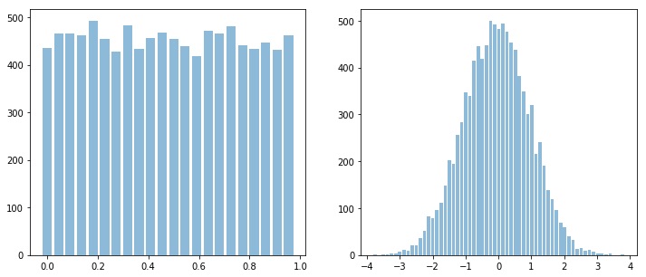
x = np.random.rand(10000)
y = np.random.randn(10000)

plt.figure(figsize=(12,5))
plt.subplot(121)
sp.HistPlot(x,show=False)

plt.subplot(122)
sp.HistPlot(y,show=False)
plt.show()

https://raw.githubusercontent.com/spkit/spkit.github.io/master/assets/images/entropy_12.jpg

Shannan entropy¶

#Shannan entropy
H_x = sp.entropy(x,alpha=1)
H_y = sp.entropy(y,alpha=1)
print('Shannan entropy')
print('Entropy of x: H(x) = ',H_x)
print('Entropy of y: H(y) = ',H_y)

Shannan entropy
Entropy of x: H(x) =  4.4581180171280685
Entropy of y: H(y) =  5.04102391756942

Rényi entropy¶

#Rényi entropy
Hr_x= sp.entropy(x,alpha=2)
Hr_y= sp.entropy(y,alpha=2)
print('Rényi entropy')
print('Entropy of x: H(x) = ',Hr_x)
print('Entropy of y: H(y) = ',Hr_y)

Rényi entropy
Entropy of x: H(x) =  4.456806796146617
Entropy of y: H(y) =  4.828391418226062

Mutual Information & Joint Entropy¶

I_xy = sp.mutual_Info(x,y)
print('Mutual Information I(x,y) = ',I_xy)

H_xy= sp.entropy_joint(x,y)
print('Joint Entropy H(x,y) = ',H_xy)

Joint Entropy H(x,y) =  9.439792556949234
Mutual Information I(x,y) =  0.05934937774825322

Conditional entropy¶

H_x1y= sp.entropy_cond(x,y)
H_y1x= sp.entropy_cond(y,x)
print('Conditional Entropy of : H(x|y) = ',H_x1y)
print('Conditional Entropy of : H(y|x) = ',H_y1x)

Conditional Entropy of : H(x|y) =  4.398768639379814
Conditional Entropy of : H(y|x) =  4.9816745398211655

Cross entropy & Kullback–Leibler divergence¶

H_xy_cross= sp.entropy_cross(x,y)
D_xy= sp.entropy_kld(x,y)
print('Cross Entropy of : H(x,y) = :',H_xy_cross)
print('Kullback–Leibler divergence : Dkl(x,y) = :',D_xy)

Cross Entropy of : H(x,y) = : 11.591688735915701
Kullback–Leibler divergence : Dkl(x,y) = : 4.203058010473213

EEG Signal¶

View in Jupyter-Notebook ¶

Single Channel¶

import numpy as np
import matplotlib.pyplot as plt
import spkit as sp
from spkit.data import load_data
print(sp.__version__)

# load sample of EEG segment
X,ch_names = load_data.eegSample()
t = np.arange(X.shape[0])/128
nC = len(ch_names)


x1 =X[:,0] #'AF3' - Frontal Lobe
x2 =X[:,6] #'O1'  - Occipital Lobe
#Shannan entropy
H_x1= sp.entropy(x1,alpha=1)
H_x2= sp.entropy(x2,alpha=1)

#Rényi entropy
Hr_x1= sp.entropy(x1,alpha=2)
Hr_x2= sp.entropy(x2,alpha=2)

print('Shannan entropy')
print('Entropy of x1: H(x1) =\t ',H_x1)
print('Entropy of x2: H(x2) =\t ',H_x2)
print('-')
print('Rényi entropy')
print('Entropy of x1: H(x1) =\t ',Hr_x1)
print('Entropy of x2: H(x2) =\t ',Hr_x2)
print('-')

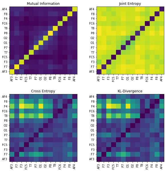
Multi-Channels (cross)¶

#Joint entropy
H_x12= sp.entropy_joint(x1,x2)

#Conditional Entropy
H_x12= sp.entropy_cond(x1,x2)
H_x21= sp.entropy_cond(x2,x1)

#Mutual Information
I_x12 = sp.mutual_Info(x1,x2)

#Cross Entropy
H_x12_cross= sp.entropy_cross(x1,x2)

#Diff Entropy
D_x12= sp.entropy_kld(x1,x2)

print('Joint Entropy H(x1,x2) =\t',H_x12)
print('Mutual Information I(x1,x2) =\t',I_x12)
print('Conditional Entropy of : H(x1|x2) =\t',H_x12)
print('Conditional Entropy of : H(x2|x1) =\t',H_x21)
print('-')
print('Cross Entropy of : H(x1,x2) =\t',H_x12_cross)
print('Kullback–Leibler divergence : Dkl(x1,x2) =\t',D_x12)


MI = np.zeros([nC,nC])
JE = np.zeros([nC,nC])
CE = np.zeros([nC,nC])
KL = np.zeros([nC,nC])
for i in range(nC):
    x1 = X[:,i]
    for j in range(nC):
        x2 = X[:,j]

        #Mutual Information
        MI[i,j] = sp.mutual_Info(x1,x2)

        #Joint entropy
        JE[i,j]= sp.entropy_joint(x1,x2)

        #Cross Entropy
        CE[i,j]= sp.entropy_cross(x1,x2)

        #Diff Entropy
        KL[i,j]= sp.entropy_kld(x1,x2)



  plt.figure(figsize=(10,10))
  plt.subplot(221)
  plt.imshow(MI,origin='lower')
  plt.yticks(np.arange(nC),ch_names)
  plt.xticks(np.arange(nC),ch_names,rotation=90)
  plt.title('Mutual Information')
  plt.subplot(222)
  plt.imshow(JE,origin='lower')
  plt.yticks(np.arange(nC),ch_names)
  plt.xticks(np.arange(nC),ch_names,rotation=90)
  plt.title('Joint Entropy')
  plt.subplot(223)
  plt.imshow(CE,origin='lower')
  plt.yticks(np.arange(nC),ch_names)
  plt.xticks(np.arange(nC),ch_names,rotation=90)
  plt.title('Cross Entropy')
  plt.subplot(224)
  plt.imshow(KL,origin='lower')
  plt.yticks(np.arange(nC),ch_names)
  plt.xticks(np.arange(nC),ch_names,rotation=90)
  plt.title('KL-Divergence')
  plt.subplots_adjust(hspace=0.3)
  plt.show()

https://raw.githubusercontent.com/spkit/spkit.github.io/master/assets/images/EEG_it3.png

Independent Component Analysis¶

Independent Component Analysis - ICA¶

View in Jupyter-Notebook ¶

import numpy as np
import matplotlib.pyplot as plt
from spkit import ICA
from spkit.data import load_data
X,ch_names = load_data.eegSample()
nC =  len(ch_names)

x = X[128*10:128*12,:]
t = np.arange(x.shape[0])/128.0

ica = ICA(n_components=nC,method='fastica')
ica.fit(x.T)
s1 = ica.transform(x.T)

ica = ICA(n_components=nC,method='infomax')
ica.fit(x.T)
s2 = ica.transform(x.T)

ica = ICA(n_components=nC,method='picard')
ica.fit(x.T)
s3 = ica.transform(x.T)

ica = ICA(n_components=nC,method='extended-infomax')
ica.fit(x.T)
s4 = ica.transform(x.T)


methods = ('fastica', 'infomax', 'picard', 'extended-infomax')
icap = ['ICA'+str(i) for i in range(1,15)]

plt.figure(figsize=(15,15))
plt.subplot(321)
plt.plot(t,x+np.arange(nC)*200)
plt.xlim([t[0],t[-1]])
plt.yticks(np.arange(nC)*200,ch_names)
plt.grid(alpha=0.3)
plt.title('X : EEG Data')

S = [s1,s2,s3,s4]
for i in range(4):
    plt.subplot(3,2,i+2)
    plt.plot(t,S[i].T+np.arange(nC)*700)
    plt.xlim([t[0],t[-1]])
    plt.yticks(np.arange(nC)*700,icap)
    plt.grid(alpha=0.3)
    plt.title(methods[i])

plt.show()

Complex Continuous Wavelet Transform¶

Complex Wavelets¶

Notebook¶

View in Jupyter-Notebook ¶

A quick example to compare different wavelets¶

import numpy as np
import matplotlib.pyplot as plt

import spkit
print('spkit-version ', spkit.__version__)
import spkit as sp
from spkit.cwt import ScalogramCWT
from spkit.cwt import compare_cwt_example

x,fs = sp.load_data.eegSample_1ch()
t = np.arange(len(x))/fs

compare_cwt_example(x,t,fs=fs)

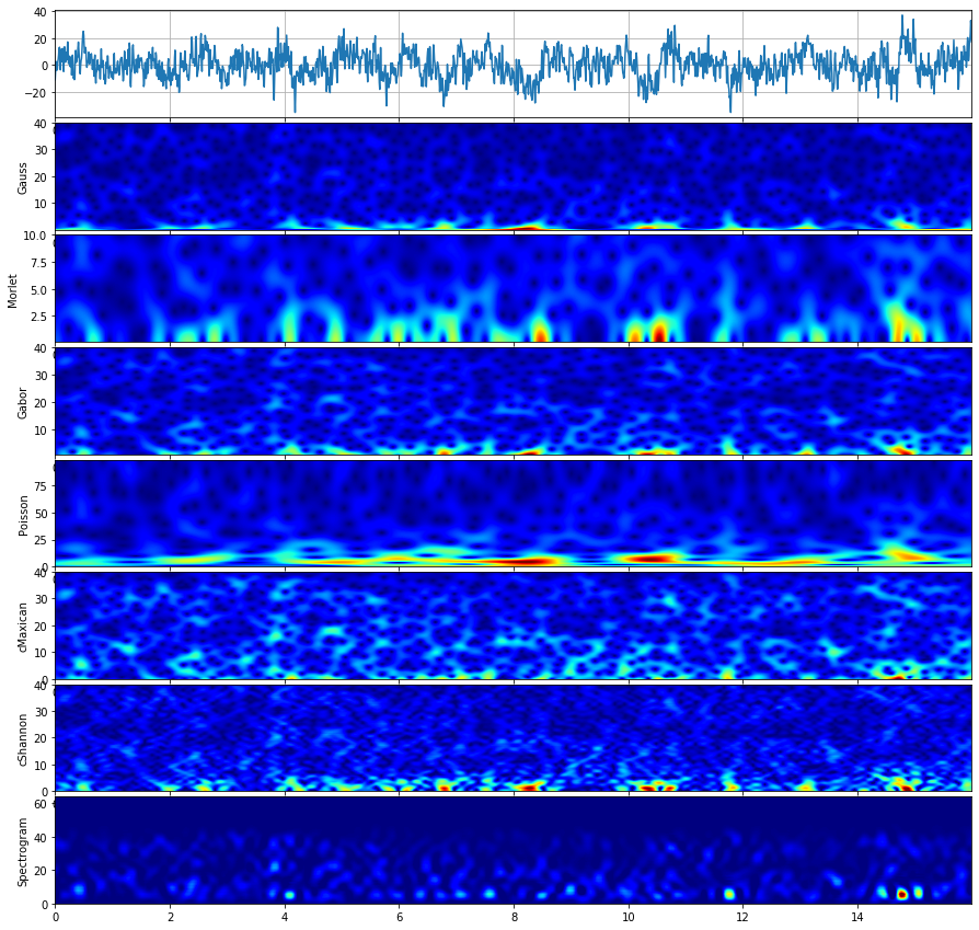
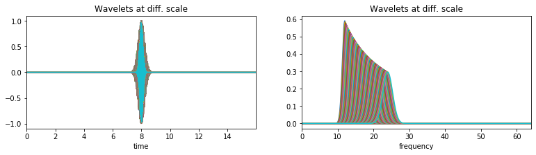
https://raw.githubusercontent.com/spkit/spkit.github.io/master/assets/images/cwt_2.png

Gauss wavelet¶

The Gauss Wavelet function in time and frequency domain are defined as $\psi(t)$ and $\psi(f)$ as below;

\[\begin{split}\psi(t) &= e^{-a(t-t_0)^{2}} \cdot e^{-2\pi jf_0(t-t_0)}\\ \psi(f) &= \sqrt{\pi/a}\left( e^{-2\pi jft_0}\cdot e^{-\pi^{2}((f-f_0)^{2})/a}\right)\end{split}\]

where

\[a = \left( \frac{f_0}{Q} \right)^{2}\]

Parameters for a Gauss wavelet:

f0 - center frequency

Q - associated with spread of bandwidth, as a = (f0/Q)^2

import numpy as np
import matplotlib.pyplot as plt

import spkit
print('spkit-version ', spkit.__version__)
import spkit as sp
from spkit.cwt import ScalogramCWT

Parameters for a Gauss wavelet:

f0 - center frequency

Q - associated with spread of bandwidth, as a = (f0/Q)^2

Plot wavelet functions¶

fs = 128                                   #sampling frequency
tx = np.linspace(-5,5,fs*10+1)             #time
fx = np.linspace(-fs//2,fs//2,2*len(tx))   #frequency range

f01 = 2     #np.linspace(0.1,5,2)[:,None]
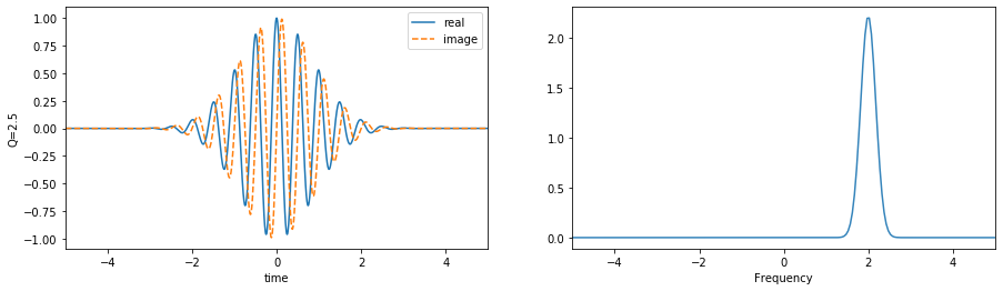
Q1  = 2.5   #np.linspace(0.1,5,10)[:,None]
wt1,wf1 = sp.cwt.GaussWave(tx,f=fx,f0=f01,Q=Q1)


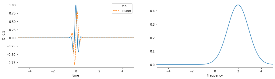
f02 = 2    #np.linspace(0.1,5,2)[:,None]
Q2  = 0.5  #np.linspace(0.1,5,10)[:,None]
wt2,wf2 = sp.cwt.GaussWave(tx,f=fx,f0=f02,Q=Q2)

plt.figure(figsize=(15,4))
plt.subplot(121)
plt.plot(tx,wt1.T.real,label='real')
plt.plot(tx,wt1.T.imag,'--',label='image')
plt.xlim(tx[0],tx[-1])
plt.xlabel('time')
plt.ylabel('Q=2.5')
plt.legend()
plt.subplot(122)
plt.plot(fx,abs(wf1.T), alpha=0.9)
plt.xlim(fx[0],fx[-1])
plt.xlim(-5,5)
plt.xlabel('Frequency')
plt.show()

plt.figure(figsize=(15,4))
plt.subplot(121)
plt.plot(tx,wt2.T.real,label='real')
plt.plot(tx,wt2.T.imag,'--',label='image')
plt.xlim(tx[0],tx[-1])
plt.xlabel('time')
plt.ylabel('Q=0.5')
plt.legend()
plt.subplot(122)
plt.plot(fx,abs(wf2.T), alpha=0.9)
plt.xlim(fx[0],fx[-1])
plt.xlim(-5,5)
plt.xlabel('Frequency')
plt.show()

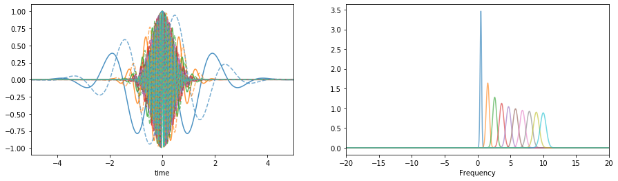
https://raw.githubusercontent.com/spkit/spkit.github.io/master/assets/images/wavelets/gauss_1.png

https://raw.githubusercontent.com/spkit/spkit.github.io/master/assets/images/wavelets/gauss_2.png

With a range of scale parameters¶

f0 = np.linspace(0.5,10,10)[:,None]
Q  = np.linspace(1,5,10)[:,None]
#Q  = 1

wt,wf = sp.cwt.GaussWave(tx,f=fx,f0=f0,Q=Q)

plt.figure(figsize=(15,4))
plt.subplot(121)
plt.plot(tx,wt.T.real, alpha=0.8)
plt.plot(tx,wt.T.imag,'--', alpha=0.6)
plt.xlim(tx[0],tx[-1])
plt.xlabel('time')
plt.subplot(122)
plt.plot(fx,abs(wf.T), alpha=0.6)
plt.xlim(fx[0],fx[-1])
plt.xlim(-20,20)
plt.xlabel('Frequency')
plt.show()

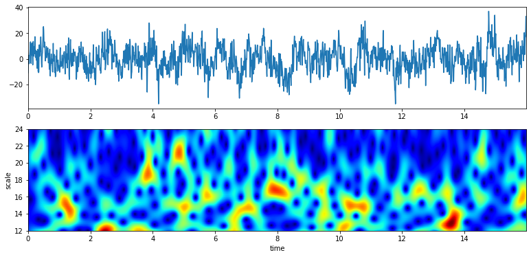
https://raw.githubusercontent.com/spkit/spkit.github.io/master/assets/images/wavelets/gauss_3_range.png

Signal Analysis - EEG¶

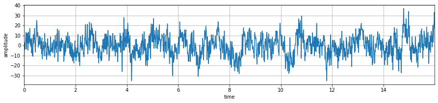
x,fs = sp.load_data.eegSample_1ch()
t = np.arange(len(x))/fs

print('shape ',x.shape, t.shape)

plt.figure(figsize=(15,3))
plt.plot(t,x)
plt.xlabel('time')
plt.ylabel('amplitude')
plt.xlim(t[0],t[-1])
plt.grid()
plt.show()

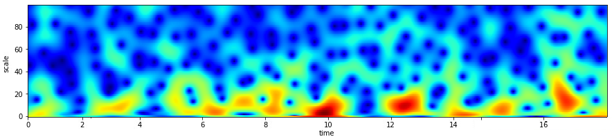
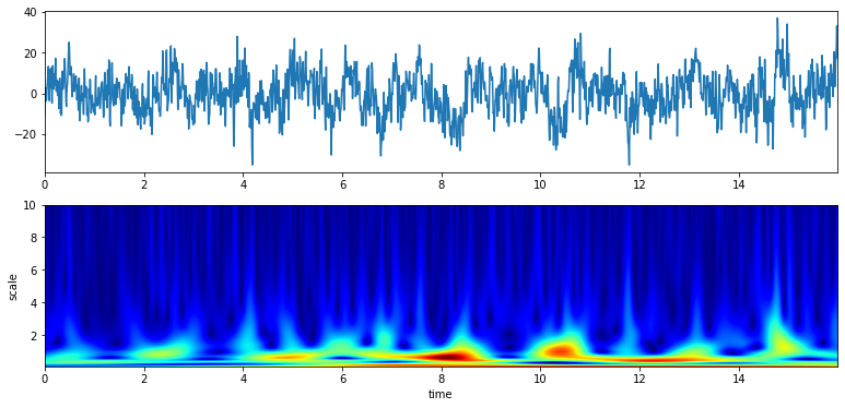
https://raw.githubusercontent.com/spkit/spkit.github.io/master/assets/images/wavelets/signal_1.png

Scalogram with default parameters¶

## With default setting of f0 and Q # f0 = np.linspace(0.1,10,100) # Q = 0.5

XW,S = ScalogramCWT(x,t,fs=fs,wType='Gauss',PlotPSD=True)

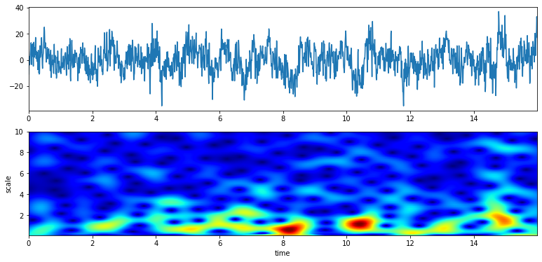
https://raw.githubusercontent.com/spkit/spkit.github.io/master/assets/images/wavelets/gauss_psd_1.png

With a range of frequency and Q¶

# from 0.1 to 10 Hz of analysis range and 100 points

f0 = np.linspace(0.1,10,100)
Q  = np.linspace(0.1,5,100)
XW,S = ScalogramCWT(x,t,fs=fs,wType='Gauss',PlotPSD=True,f0=f0,Q=Q)

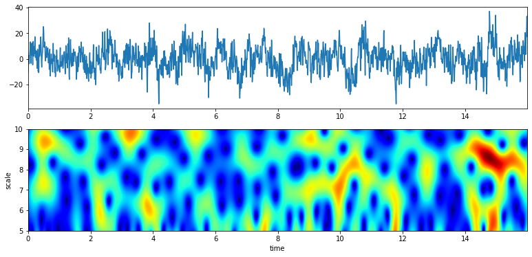
https://raw.githubusercontent.com/spkit/spkit.github.io/master/assets/images/wavelets/gauss_psd_2.png

# from 5 to 10 Hz of analysis range and 100 points

f0 = np.linspace(5,10,100)
Q  = np.linspace(1,4,100)
XW,S = ScalogramCWT(x,t,fs=fs,wType='Gauss',PlotPSD=True,f0=f0,Q=Q)

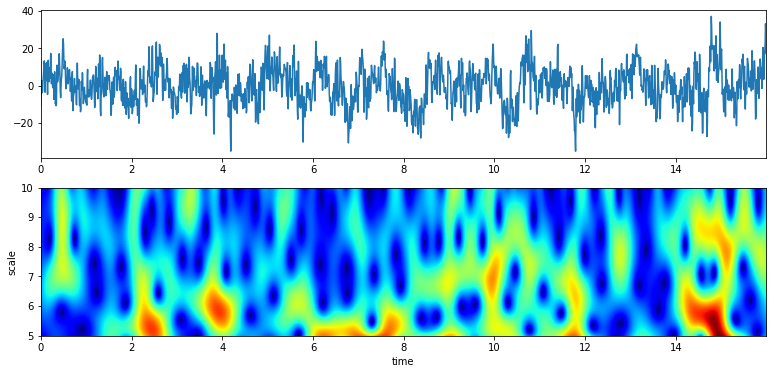
https://raw.githubusercontent.com/spkit/spkit.github.io/master/assets/images/wavelets/gauss_psd_3.png

# With constant Q

f0 = np.linspace(5,10,100)
Q  = 2
XW,S = ScalogramCWT(x,t,fs=fs,wType='Gauss',PlotPSD=True,f0=f0,Q=Q)

https://raw.githubusercontent.com/spkit/spkit.github.io/master/assets/images/wavelets/gauss_psd_4.png

# From 12 to 24 Hz

f0 = np.linspace(12,24,100)
Q  = 4
XW,S = ScalogramCWT(x,t,fs=fs,wType='Gauss',PlotPSD=True,f0=f0,Q=Q)

https://raw.githubusercontent.com/spkit/spkit.github.io/master/assets/images/wavelets/gauss_psd_5.png

With a plot of analysis wavelets¶

f0 = np.linspace(12,24,100)
Q  = 4
XW,S = ScalogramCWT(x,t,fs=fs,wType='Gauss',PlotPSD=True,PlotW=True, f0=f0,Q=Q)

https://raw.githubusercontent.com/spkit/spkit.github.io/master/assets/images/wavelets/gauss_psd_6_1.png

https://raw.githubusercontent.com/spkit/spkit.github.io/master/assets/images/wavelets/gauss_psd_6_2.png

#TODO Speech/Audio Signal

Speech¶

#TODO

Audio¶

#TODO

Morlet wavelet¶

#TODO

The Morlet Wavelet function in time and frequency domain are defined as $\psi(t)$ and $\psi(f)$ as below;

\[\begin{split}\psi(t) &= C_{\sigma}\pi^{-0.25} e^{-0.5t^2} \left(e^{j\sigma t}-K_{\sigma} \right)\\ \psi(w) &= C_{\sigma}\pi^{-0.25} \left(e^{-0.5(\sigma-w)^2} -K_{\sigma}e^{-0.5w^2} \right)\end{split}\]

where

\[\begin{split}C_{\sigma} &= \left(1+ e^{-\sigma^{2}} - 2e^{-\frac{3}{4}\sigma^{2}} \right)^{-0.5}\\ K_{\sigma} &=e^{-0.5\sigma^{2}}\\ w &= 2\pi f\end{split}\]

Gabor wavelet¶

#TODO

The Gabor Wavelet function (technically same as Gaussian) in time and frequency domain are defined as $\psi(t)$ and $\psi(f)$ as below;

\[\begin{split}\psi(t) &= e^{-(t-t_0)^2/a^2}e^{-jf_0(t-t_0)}\\ \psi(f) &= e^{-((f-f_0)a)^2}e^{-jt_0(f-f_0)}\end{split}\]

where $a$ is oscilation rate and $f_0$ is center frequency

Poisson wavelet¶

Poisson wavelet is defined by positive integers ($n$), unlike other, and associated with Poisson probability distribution

The Poisson Wavelet function in time and frequency domain are defined as $\psi(t)$ and $\psi(f)$ as below;

#Type 1 (n)¶

\[\begin{split}\psi(t) &= \left(\frac{t-n}{n!}\right)t^{n-1} e^{-t}\\ \psi(w) &= \frac{-jw}{(1+jw)^{n+1}}\end{split}\]

where

Admiddibility const $C_{\psi} =\frac{1}{n}$ and $w = 2\pi f$

#Type 2¶

\[\begin{split}\psi(t) &= \frac{1}{\pi} \frac{1-t^2}{(1+t^2)^2}\\ \psi(t) &= p(t) + \frac{d}{dt}p(t)\\ \psi(w) &= |w|e^{-|w|}\end{split}\]

where

\[\begin{split}p(t) &=\frac{1}{\pi}\frac{1}{1+t^2}\\ w &= 2\pi f\end{split}\]

#Type 3 (n)¶

\[\begin{split}\psi(t) &= \frac{1}{2\pi}(1-jt)^{-(n+1)}\\ \psi(w) &= \frac{1}{\Gamma{n+1}}w^{n}e^{-w}u(w)\end{split}\]

where

\[\begin{split}\text{unit step function }\quad u(w) &=1 \quad \text{ if $w>=0$ }\quad \text{else } 0\\ w &= 2\pi f\end{split}\]

#TODO

Maxican wavelet¶

Complex Mexican hat wavelet is derived from the conventional Mexican hat wavelet. It is a low-oscillation wavelet which is modulated by a complex exponential function with frequency $f_0$ Ref..

The Maxican Wavelet function in time and frequency domain are defined as $\psi(t)$ and $\psi(f)$ as below;

\[\begin{split}\psi(t) &= \frac{2}{\sqrt{3}} \pi^{-\frac{1}{4}}\left(\sqrt{\pi}(1-t^2)e^{-\frac{1}{2}t^2} - \left(\sqrt{2}jt + \sqrt{\pi}erf\left[\frac{j}{\sqrt{2}}t \right] (1-t^2)e^{-\frac{1}{2}t^2}\right)\right)e^{-2\pi jf_0 t}\\\\ \psi(w) &= 2\sqrt{\frac{2}{3}}\pi^{-1/4}(w-w_0)^2e^{-\frac{1}{2} (w-w_0)^2} \quad \text{ if $w\ge 0$,}\quad \text{ 0 else}\end{split}\]

where $w = 2\pi f$ and $w_0 = 2\pi f_0$

#TODO

Shannon wavelet¶

Complex Shannon wavelet is the most simplified wavelet function, exploiting Sinc function by modulating with sinusoidal, which results in an ideal bandpass filter. Real Shannon wavelet is modulated by only a cos function Ref.

The Shannon Wavelet function in time and frequency domain are defined as $\psi(t)$ and $\psi(f)$ as below;

\[\begin{split}\psi(t) &= Sinc(t/2) \cdot e^{-2j\pi f_0t}\\ \psi(w) &= \prod \left( \frac{w-w_0}{\pi} \right)\end{split}\]

where

where $\prod (x) = 1$ if $x \leq 0.5$, 0 else and $w = 2\pi f$ and $w_0 = 2\pi f_0$

#TODO

Machine Learning¶

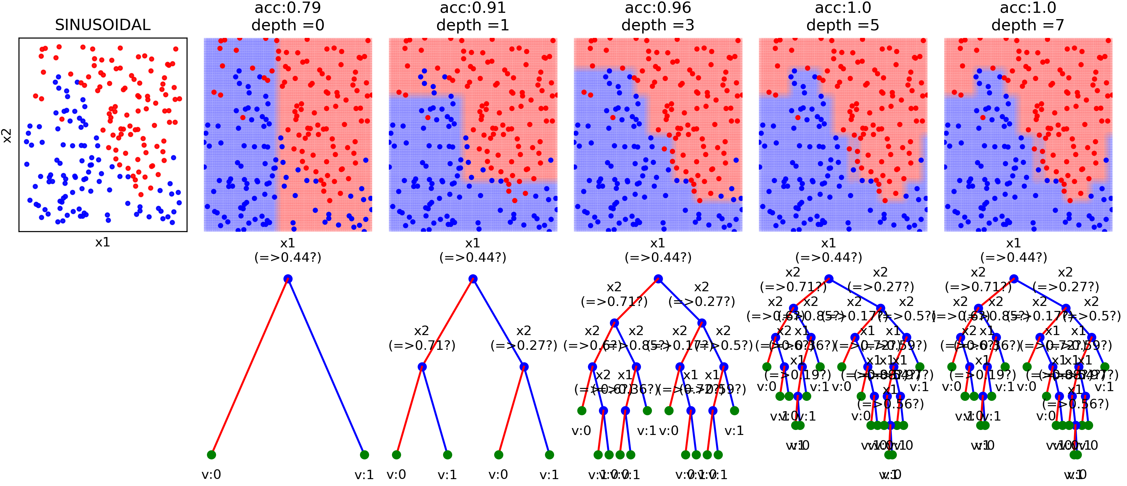
New Updates¶

Decision Tree - View Notebooks ¶

Version: 0.0.9:
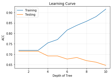
Analysing the performance measure of trained tree at different depth - with ONE-TIME Training ONLY
Optimize the depth of tree
Shrink the trained tree with optimal depth
Plot the Learning Curve
Classification: Compute the probability and counts of label at a leaf for given example sample
Regression: Compute the standard deviation and number of training samples at a leaf for given example sample

https://raw.githubusercontent.com/Nikeshbajaj/spkit/master/figures/DTree_withKDepth1.png

https://raw.githubusercontent.com/Nikeshbajaj/spkit/master/figures/DTree_LCurve.png

Version: 0.0.6: Works with catogorical features without converting them into binary vector
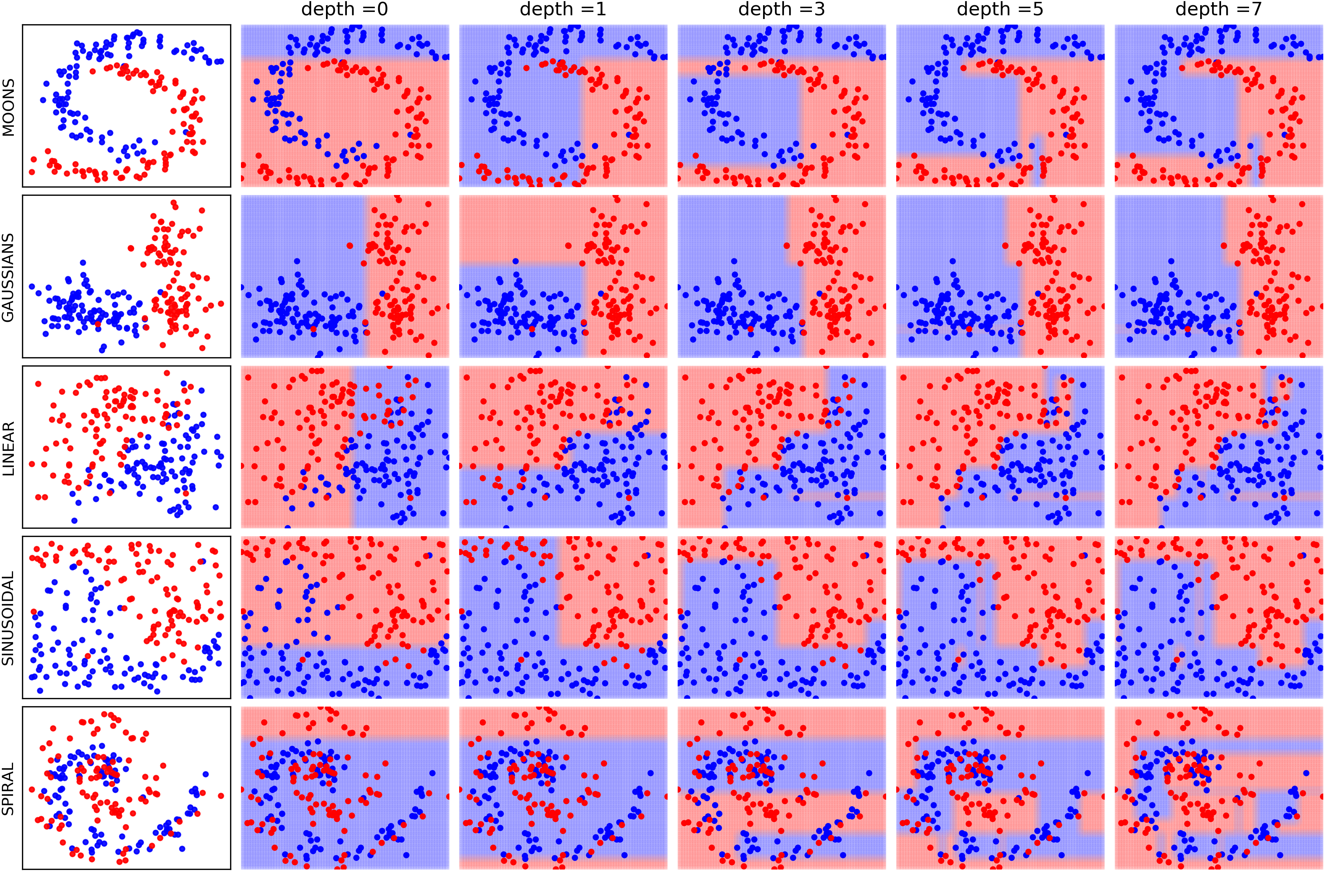
Version: 0.0.5: Toy examples to understand the effect of incresing max_depth of Decision Tree

https://raw.githubusercontent.com/Nikeshbajaj/spkit/master/figures/DTree_withCatogoricalFeatures.png

https://raw.githubusercontent.com/Nikeshbajaj/spkit/master/figures/tree_sinusoidal.png

Logistic Regression¶

View more examples in Notebooks ¶

https://raw.githubusercontent.com/Nikeshbajaj/MachineLearningFromScratch/master/LogisticRegression/img/example1.gif

Binary Class¶

import numpy as np
import matplotlib.pyplot as plt

import spkit
print(spkit.__version__)
0.0.9

from spkit.ml import LogisticRegression

# Generate data
N = 300
np.random.seed(1)
X = np.random.randn(N,2)
y = np.random.randint(0,2,N)
y.sort()

X[y==0,:]+=2 # just creating classes a little far
print(X.shape, y.shape)
plt.plot(X[y==0,0],X[y==0,1],'.b')
plt.plot(X[y==1,0],X[y==1,1],'.r')
plt.show()


clf = LogisticRegression(alpha=0.1)
print(clf)
clf.fit(X,y,max_itr=1000)
yp  = clf.predict(X)
ypr = clf.predict_proba(X)
print('Accuracy : ',np.mean(yp==y))
print('Loss     : ',clf.Loss(y,ypr))

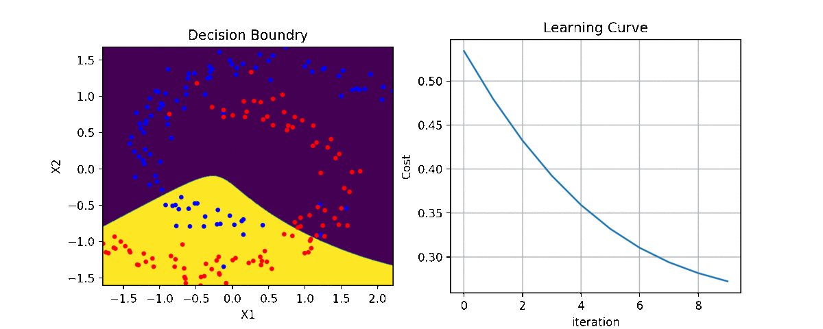
plt.figure(figsize=(12,7))
ax1 = plt.subplot(221)
clf.plot_Lcurve(ax=ax1)
ax2 = plt.subplot(222)
clf.plot_boundries(X,y,ax=ax2)

ax3 = plt.subplot(223)
clf.plot_weights(ax=ax3)
ax4 = plt.subplot(224)
clf.plot_weights2(ax=ax4,grid=False)

Multi Class - with polynomial features¶

N =300
X = np.random.randn(N,2)
y = np.random.randint(0,3,N)
y.sort()

X[y==0,1]+=3
X[y==2,0]-=3
print(X.shape, y.shape)

plt.plot(X[y==0,0],X[y==0,1],'.b')
plt.plot(X[y==1,0],X[y==1,1],'.r')
plt.plot(X[y==2,0],X[y==2,1],'.g')
plt.show()

clf = LogisticRegression(alpha=0.1,polyfit=True,degree=3,lambd=0,FeatureNormalize=True)
clf.fit(X,y,max_itr=1000)
yp  = clf.predict(X)
ypr = clf.predict_proba(X)
print(clf)
print('')
print('Accuracy : ',np.mean(yp==y))
print('Loss     : ',clf.Loss(clf.oneHot(y),ypr))


plt.figure(figsize=(15,7))
ax1 = plt.subplot(221)
clf.plot_Lcurve(ax=ax1)
ax2 = plt.subplot(222)
clf.plot_boundries(X,y,ax=ax2)

ax3 = plt.subplot(223)
clf.plot_weights(ax=ax3)
ax4 = plt.subplot(224)
clf.plot_weights2(ax=ax4,grid=True)

Naive Bayes¶

View more examples in Notebooks ¶

https://raw.githubusercontent.com/Nikeshbajaj/MachineLearningFromScratch/master/Probabilistic/img/FeatureDist.png

import numpy as np
import matplotlib.pyplot as plt

#for dataset and splitting
from sklearn import datasets
from sklearn.model_selection import train_test_split


from spkit.ml import NaiveBayes

#Data
data = datasets.load_iris()
X = data.data
y = data.target

Xt,Xs,yt,ys = train_test_split(X,y,test_size=0.3)

print('Data Shape::',Xt.shape,yt.shape,Xs.shape,ys.shape)

#Fitting
clf = NaiveBayes()
clf.fit(Xt,yt)

#Prediction
ytp = clf.predict(Xt)
ysp = clf.predict(Xs)

print('Training Accuracy : ',np.mean(ytp==yt))
print('Testing  Accuracy : ',np.mean(ysp==ys))


#Probabilities
ytpr = clf.predict_prob(Xt)
yspr = clf.predict_prob(Xs)
print('\nProbability')
print(ytpr[0])

#parameters
print('\nParameters')
print(clf.parameters)


#Visualising
clf.set_class_labels(data['target_names'])
clf.set_feature_names(data['feature_names'])


fig = plt.figure(figsize=(10,8))
clf.VizPx()

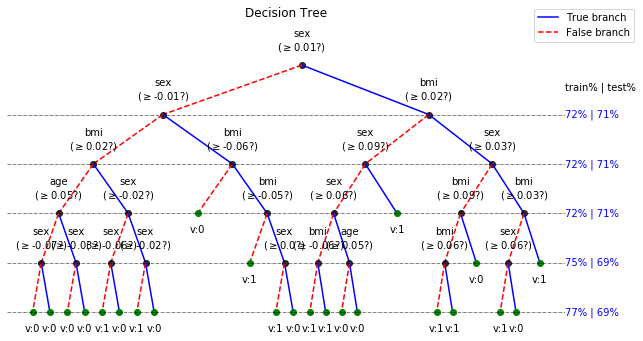
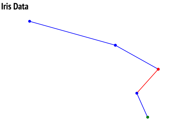
Decision Trees¶

View more examples in Notebooks ¶

Or just execute all the examples online, without installing anything

One example file is

import numpy as np
import matplotlib.pyplot as plt

# Data and Split
from sklearn.model_selection import train_test_split
from sklearn.datasets import load_diabetes

from spkit.ml import ClassificationTree


data = load_diabetes()
X = data.data
y = 1*(data.target>np.mean(data.target))

feature_names = data.feature_names
print(X.shape, y.shape)
Xt,Xs,yt,ys = train_test_split(X,y,test_size =0.3)
print(Xt.shape, Xs.shape,yt.shape, ys.shape)


clf = ClassificationTree(max_depth=7)
clf.fit(Xt,yt,feature_names=feature_names)
ytp = clf.predict(Xt)
ysp = clf.predict(Xs)

ytpr = clf.predict_proba(Xt)[:,1]
yspr = clf.predict_proba(Xs)[:,1]

print('Depth of trained Tree ', clf.getTreeDepth())
print('Accuracy')
print('- Training : ',np.mean(ytp==yt))
print('- Testing  : ',np.mean(ysp==ys))
print('Logloss')
Trloss = -np.mean(yt*np.log(ytpr+1e-10)+(1-yt)*np.log(1-ytpr+1e-10))
Tsloss = -np.mean(ys*np.log(yspr+1e-10)+(1-ys)*np.log(1-yspr+1e-10))
print('- Training : ',Trloss)
print('- Testing  : ',Tsloss)

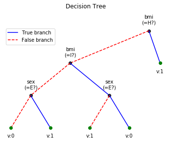
# Plot Tree
plt.figure(figsize=(15,12))
clf.plotTree()

Depth Analysis¶

View more examples in Notebooks

https://raw.githubusercontent.com/Nikeshbajaj/spkit/master/figures/trees.png

Plottng tree while training¶

https://raw.githubusercontent.com/Nikeshbajaj/MachineLearningFromScratch/master/Trees/img/a123_nik.gif

LFSR¶

Link to pylfsr documentation¶

Example: 5 bit LFSR with x^5 + x^2 + 1¶

import numpy as np
from spkit.pylfsr import LFSR

L = LFSR()
L.info()
L.next()
L.runKCycle(10)
L.runFullCycle()
L.info()
tempseq = L.runKCycle(10000)    # generate 10000 bits from current state

Check out full documentation of LFSR**¶

https://lfsr.readthedocs.io/

Contacts¶

If any doubt, confusion or feedback please contact me at

n.bajaj@qmul.ac.uk
nikkeshbajaj@gmail.com

Nikesh Bajaj: http://nikeshbajaj.in PhD Student: Queen Mary University of London

Signal Processing Toolkit - Documentation!¶

Homepage spkit - https://spkit.github.io¶

Getting started¶

Links:¶

Installation¶

Information Theory¶

Information Theory for Real-Valued signals¶

Entropy of real-valued signal¶

Shannan entropy¶

Rényi entropy¶

Mutual Information & Joint Entropy¶

Conditional entropy¶

Cross entropy & Kullback–Leibler divergence¶

EEG Signal¶

Single Channel¶

Multi-Channels (cross)¶

Independent Component Analysis¶

Independent Component Analysis - ICA¶

Complex Continuous Wavelet Transform¶

Complex Wavelets¶

Notebook¶

A quick example to compare different wavelets¶

Gauss wavelet¶

Plot wavelet functions¶

With a range of scale parameters¶

Signal Analysis - EEG¶

Scalogram with default parameters¶

With a range of frequency and Q¶

With a plot of analysis wavelets¶

Speech¶

Audio¶

Morlet wavelet¶

Gabor wavelet¶

Poisson wavelet¶

#Type 1 (n)¶

#Type 2¶

#Type 3 (n)¶

Maxican wavelet¶

Shannon wavelet¶

Machine Learning¶

Machine Learning¶

New Updates¶

Logistic Regression¶

Binary Class¶

Multi Class - with polynomial features¶

Naive Bayes¶

Decision Trees¶

Depth Analysis¶

Plottng tree while training¶

LFSR¶

Link to pylfsr documentation¶

Example: 5 bit LFSR with x^5 + x^2 + 1¶

Contacts¶

Contacts¶

Homepage spkit - https://spkit.github.io ¶