Dispersion Entropy
Backgorund
Unlike usual entropy, Dispersion Entropy take the temporal dependency into accounts, same as Sample Entropy and Aproximate Entropy. It is Embeding Based Entropy function. The idea of Dispersion is almost same as Sample and Aproximate, which is to extract Embeddings, estimate their distribuation and compute entropy. However, there is a fine detail that make dispersion entropy more usuful.
First, is to map the distribuation original signal to uniform (using CDF), then divide them into n-classes. This is same as done for quantization process of any normally distributed signal, such as speech. In quantization, this mapping helps to minimize the quantization error, by assiging small quantization steps for samples with high density and large for low. Think this in a way, if in a signal, large number of samples belongs to a range (-0.1, 0.1), near to zero, your almost all the embeddings will have at least one value that is in that range. CDF mapping will avoid that. In this python implimentation, we have included other mapping functions, which are commonly used in speech processing, i.e. A-Law, and µ-Law, with parameter A and µ to control the mapping.
Second, it allows to extract Embedding with delay factor, i.e. if delay is 2, an embeding is continues samples skiping everu other sample. which is kind of decimation. This helps if your signal is sampled at very high sampling frequecy, i.e. super smooth in local region. Consider you hhave a signal with very high smapling rate, then many of the continues samples will have similar values, which will lead to have a very high number of contant embeddings.
Third, actuall not so much of third, but an alternative to deal with signal with very high sampling rate, is by scale factor, which is nothing but a decimator.
An Example
import numpy as np
import matplotlib.pyplot as plt
import spkit as sp

X,ch_names = sp.load_data.eegSample()
fs=128

#filtering
Xf = sp.filter_X(X,band=[1,20],btype='bandpass',verbose=0)

Xi = Xf[:,0].copy() # only one channel

de,prob,patterns_dict,_,_= sp.dispersion_entropy(Xi,classes=10, scale=1, emb_dim=2, delay=1,return_all=True)
print(de)
2.271749287746759
Important Note: Log base
The Entropy here is computed as \(-\sum p(x)log_e (p(x))\) , natural log. To convert to log2, simply divide the value with np.log(2)
de/np.log(2)
3.2774414315752844
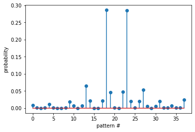
Probability of all the patterns found
plt.stem(prob)
plt.xlabel('pattern #')
plt.ylabel('probability')
plt.show()
Pattern dictionary
patterns_dict
{(1, 1): 18,
 (1, 2): 2,
 (1, 4): 1,
 (2, 1): 2,
 (2, 2): 23,
 (2, 3): 2,
 (2, 5): 1,
 (3, 1): 1,
 (3, 2): 2,
top 10 patters
PP = np.array([list(k)+[patterns_dict[k]] for k in patterns_dict])
idx = np.argsort(PP[:,-1])[::-1]
PP[idx[:10],:-1]
array([[ 5,  5],
       [ 6,  6],
       [ 4,  4],
       [ 7,  7],
       [ 6,  5],
       [ 5,  6],
       [10, 10],
       [ 4,  5],
       [ 5,  4],
       [ 8,  8]], dtype=int64)
Embedding diamension 4
de,prob,patterns_dict,_,_= sp.dispersion_entropy(Xi,classes=20, scale=1, emb_dim=4, delay=1,return_all=True)
de
4.86637389336799
top 10 patters
PP = np.array([list(k)+[patterns_dict[k]] for k in patterns_dict])
idx = np.argsort(PP[:,-1])[::-1]
PP[idx[:10],:-1]
array([[10, 10, 10, 10],
       [11, 11, 11, 11],
       [12, 12, 12, 12],
       [ 9,  9,  9,  9],
       [11, 11, 10, 10],
       [10, 10, 11, 11],
       [11, 11, 11, 10],
       [10, 10, 10, 11],
       [10, 11, 11, 11],
       [11, 10, 10, 10]], dtype=int64)
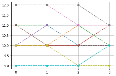
top-10, non-constant pattern
Ptop = np.array(list(PP[idx,:-1]))
idx2 = np.where(np.sum(np.abs(Ptop-Ptop.mean(1)[:,None]),1)>0)[0]
plt.plot(Ptop[idx2[:10]].T,'--o')
plt.xticks([0,1,2,3])
plt.grid()
plt.show()
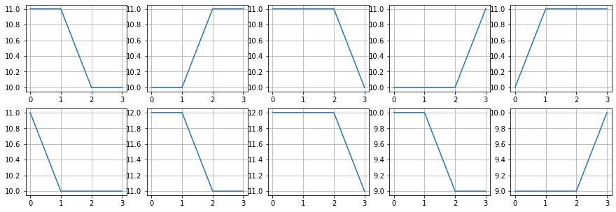
plt.figure(figsize=(15,5))
for i in range(10):
     plt.subplot(2,5,i+1)
     plt.plot(Ptop[idx2[i]])
     plt.grid()
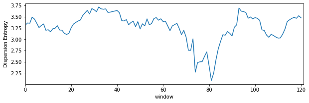
Dispersion Entropy with sliding window
de_temporal = []
win = np.arange(128)
while win[-1]<Xi.shape[0]:
    de,_ = sp.dispersion_entropy(Xi[win],classes=10, scale=1, emb_dim=2, delay=1,return_all=False)
    win+=16
    de_temporal.append(de)x


plt.figure(figsize=(10,3))
plt.plot(de_temporal)
plt.xlim([0,len(de_temporal)])
plt.xlabel('window')
plt.ylabel('Dispersion Entropy')
plt.show()
Dispersion Entropy multiscale
for scl in [1,2,3,5,10,20,30]:
   de,_ = sp.dispersion_entropy(Xi,classes=10, scale=scl, emb_dim=2, delay=1,return_all=False)
   print(f'Sacle: {scl}, \t: DE: {de}')
Sacle: 1,    : DE: 2.271749287746759
Sacle: 2,    : DE: 2.5456280627759336
Sacle: 3,    : DE: 2.6984938704051236
Sacle: 5,    : DE: 2.682837351130069
Sacle: 10,   : DE: 2.5585556625642476
Sacle: 20,   : DE: 2.7480275694000103
Sacle: 30,   : DE: 2.4767472897625806
help(sp.dispersion_entropy)
Multiscale-refined Dispersion Entropy
de,_ = sp.dispersion_entropy_multiscale_refined(Xi,classes=10, scales=[1, 2, 3, 4, 5], emb_dim=2, delay=1)
print(de)
2.543855087400606
help(sp.dispersion_entropy_multiscale_refined)