EEG Topographic Maps

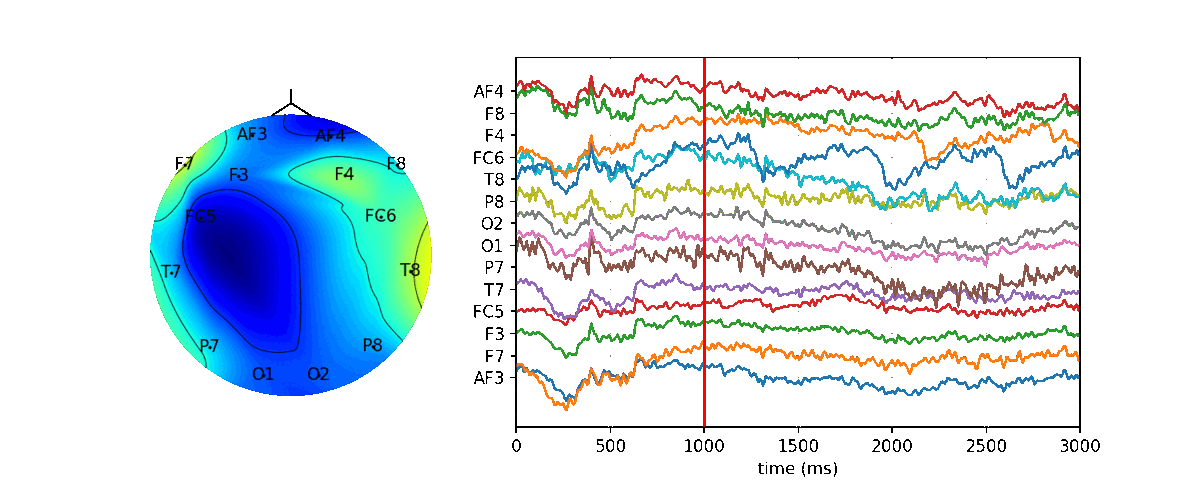
Spatio-Temporal Map

At t=0, X[0]

import spkit as sp
import matplotlib.pyplot as plt

X,ch_names = sp.load_data.eegSample()
fs=128

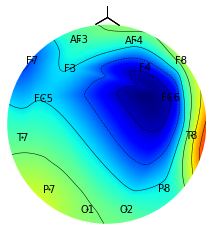
Zi = sp.eeg.TopoMap(pos,X[0],res=128, showplot=True,axes=None,contours=True,showsensors=True,
            interpolation=None,shownames=True, ch_names=ch_names,showhead=True,vmin=None,vmax=None,
            returnIm = False,fontdict=None)
plt.show()

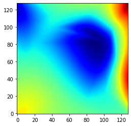
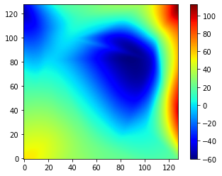
plt.imshow(Zi,cmap='jet',origin='lower')

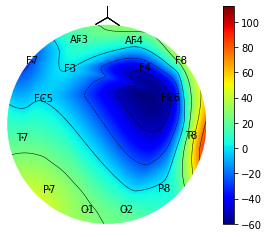
With Colorbar as voltage

import numpy as np
import matplotlib.pyplot as plt
import spkit as sp

X,ch_names = sp.load_data.eegSample()


Zi,im = sp.eeg.TopoMap(pos,X[0],res=128, showplot=True,axes=None,contours=True,showsensors=True,
            interpolation=None,shownames=True, ch_names=ch_names,showhead=True,vmin=None,vmax=None,
            returnIm = True,fontdict=None)

plt.colorbar(im)
plt.show()

im = plt.imshow(Zi,cmap='jet',origin='lower')
plt.colorbar(im)
plt.show()

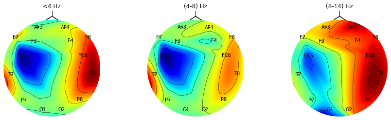
Spatio-Spectral Map

For Three different frequency Bands

fBands =[[4],[4,8],[8,14]]
Px = sp.eeg.RhythmicDecomposition(X,fs=128.0,order=5,Sum=True,Mean=False,SD=False,fBands=fBands)[0]
Px = 10*np.log10(Px)

fig = plt.figure(figsize=(15,4))
ax1 = fig.add_subplot(131)
Zi  = sp.eeg.TopoMap(pos,Px[0],res=128, showplot=True,axes=ax1,ch_names=ch,vmin=None,vmax=None)
ax1.set_title('<4 Hz')

ax2 = fig.add_subplot(132)
Zi  = sp.eeg.TopoMap(pos,Px[1],res=128, showplot=True,axes=ax2,ch_names=ch,vmin=None,vmax=None)
ax2.set_title('(4-8) Hz')

ax3 = fig.add_subplot(133)
Zi  = sp.eeg.TopoMap(pos,Px[2],res=128, showplot=True,axes=ax3,ch_names=ch,vmin=None,vmax=None)
ax3.set_title('(8-14) Hz')
plt.show()

*Note that colorbar is not shown, and power in each band has different range*

Spatio-Spectro-Temporal Map

Spatio-Spectral Map

According to Parseval’s theorem, energy in time-domain and frequency domain remain same, so computing total power at each channel for 1 sec with 0.5 overlapping

%matplotlib notebook
N = 128
skip = 32
diff = 50

tx = 1000*np.arange(X.shape[0])/fs

fig, (ax1, ax2) = plt.subplots(1, 2, figsize=(10,4),gridspec_kw={'width_ratios': [1,2]})

for i in range(0,len(X)-N,skip):
    ax1.clear()
    ee = np.sqrt(np.abs(X[i:i+N,:]).sum(0))
    _ = sp.eeg.TopoMap(pos,ee,res=128, showplot=True,axes=ax1,contours=True,showsensors=True,
            interpolation=None,shownames=True, ch_names=ch_names,showhead=True,vmin=None,vmax=None,
            returnIm = False,fontdict=None)

    ax2.clear()
    ax2.plot(tx[i:i+3*N],X[i:i+3*N,:] + diff*np.arange(14))
    ax2.set_yticks(diff*np.arange(14))
    ax2.set_yticklabels(ch_names)
    ax2.set_xlabel('time (ms)')
    ax2.set_xlim([tx[i],tx[i+3*N]])
    ax2.grid(alpha=0.4)
    ax2.axvline(tx[i+N],color='r')
    fig.canvas.draw()