ATAR - Automatic and Tunable Artifact Removal Algorithm for EEG¶

Notebook¶

View in Jupyter-Notebook ¶

ATAR Algorithm - Automatic and Tunable Artifact Removal Algorithm for EEG Signal.

The algorithm is based on wavelet packet decomposion (WPD), the full description of algorithm can be found here **Automatic and Tunable Artifact Removal Algorithm for EEG** from the article. The algorithm is applied on the given multichannel signal X (n,nch), window wise and reconstructed with overall add method. The defualt window size is set to 1 sec (128 samples). For each window, the threshold $theta_alpha$ is computed and applied to filter the wavelet coefficients. There is manily one parameter that can be tuned $beta$ with different operating modes and other settings. Here is the list of parameters and there simplified meaning given: Parameters: * $beta$: This is a main parameter to tune, highher the value, more aggressive the algorithm to remove the artifacts. By default it is set to 0.1. $beta$ is postive float value. * *OptMode*: This sets the mode of operation, which decides hoe to remove the artifact. By default it is set to ‘soft’, which means Soft Thresholding, in this mode, rather than removing the pressumed artifact, it is suppressed to the threshold, softly. OptMode=’linAtten’, suppresses the pressumed artifact depending on how far it is from threshold. Finally, the most common mode - Elimination (OptMode=’elim’), which remove the pressumed artifact.

Soft Thresholding and Linear Attenuation require addition parameters to set the associated thresholds which are by default set to bf=2, gf=0.8.

Soft Thresholding

Linear Attenuation

Elimination

*wv=db3*: Wavelet funtion, by default set to db3, could be any of [‘db3’…..’db38’, ‘sym2…..sym20’, ‘coif1…..coif17’, ‘bior1.1….bior6.8’, ‘rbio1.1…rbio6.8’, ‘dmey’]
$k_1$, $k_2$: Lower and upper bounds on threshold $theta_alpha$.
*IPR=[25,75]*: interpercentile range, range used to compute threshold

APIs

There are three functions in spkit.eeg for ATAR algorithm

spkit.eeg.ATAR_1Ch(…)
spkit.eeg.ATAR_mCh(…)
spkit.eeg.ATAR_mCh_noParallel(…)

*sp.eeg.ATAR_1Ch* is for single channel input signal x of shape (n,), where as, *sp.eeg.ATAR_mCh* is for multichannel signal X with shape (n,ch), which uses joblib for parallel processing of multi channels. For some OS, joblib raise an error of *BrokenProcessPool*, in that case use *sp.eeg.ATAR_mCh_noParallel*, which is same as *sp.eeg.ATAR_mCh*, except parallel processing. Alternatively, use *sp.eeg.ATAR_1Ch* with for loop for each channel.

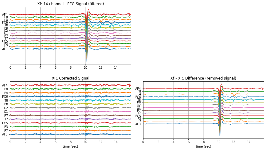
https://raw.githubusercontent.com/Nikeshbajaj/spkit/master/figures/atar_beta_tune.gif

(1) Soft Thresholding (𝛽=0.1) - a quick example¶

import numpy as np
import matplotlib.pyplot as plt

import spkit as sp
from spkit.data import load_data

print(sp.__version__)

X,ch_names = load_data.eegSample()
fs = 128

# high=pass filtering
Xf = sp.filter_X(X,band=[0.5], btype='highpass',fs=fs,verbose=0).T
Xf.shape

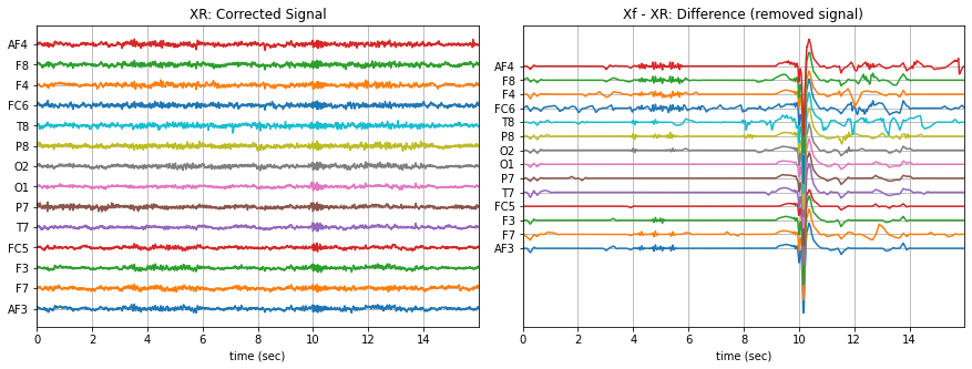
# ATAR Algorithm - default mode is 'soft' and beta=0.1
XR = sp.eeg.ATAR_mCh_noParallel(Xf.copy(),verbose=0)

#plots
t = np.arange(Xf.shape[0])/fs
plt.figure(figsize=(15,8))
plt.subplot(221)
plt.plot(t,Xf+np.arange(-7,7)*200)
plt.xlim([t[0],t[-1]])
#plt.xlabel('time (sec)')
plt.yticks(np.arange(-7,7)*200,ch_names)
plt.grid()
plt.title('Xf: 14 channel - EEG Signal (filtered)')
plt.subplot(223)
plt.plot(t,XR+np.arange(-7,7)*200)
plt.xlim([t[0],t[-1]])
plt.xlabel('time (sec)')
plt.yticks(np.arange(-7,7)*200,ch_names)
plt.grid()
plt.title('XR: Corrected Signal')
plt.subplot(224)
plt.plot(t,(Xf-XR)+np.arange(-7,7)*200)
plt.xlim([t[0],t[-1]])
plt.xlabel('time (sec)')
plt.yticks(np.arange(-7,7)*200,ch_names)
plt.grid()
plt.title('Xf - XR: Difference (removed signal)')
plt.subplots_adjust(wspace=0.1,hspace=0.3)
plt.show()

https://raw.githubusercontent.com/Nikeshbajaj/spkit/master/figures/atar_exp1.png

(2) Linear Attenuation¶

XR = sp.eeg.ATAR_mCh_noParallel(Xf.copy(),verbose=0,OptMode='linAtten')

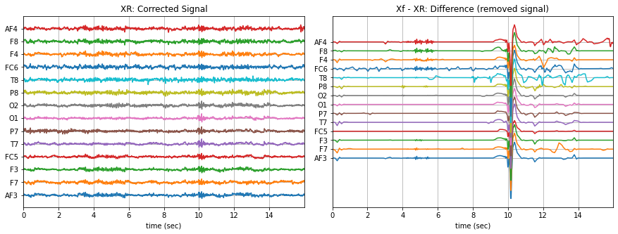
https://raw.githubusercontent.com/Nikeshbajaj/spkit/master/figures/atar_exp2_linAtten.png

(3) Elimination¶

XR = sp.eeg.ATAR_mCh_noParallel(Xf.copy(),verbose=0,OptMode='elim')

https://raw.githubusercontent.com/Nikeshbajaj/spkit/master/figures/atar_exp3_elim.png

Tuning 𝛽 with ‘soft’ : Controlling the aggressiveness¶

betas = np.r_[np.arange(0.01,0.1,0.02), np.arange(0.1,1.1, 0.1)].round(2)

for b in betas:
    XR = sp.eeg.ATAR_mCh_noParallel(Xf.copy(),verbose=0,beta=b,OptMode='soft')
    XR.shape

    plt.figure(figsize=(15,5))
    plt.subplot(121)
    plt.plot(t,XR+np.arange(-7,7)*200)
    plt.xlim([t[0],t[-1]])
    plt.xlabel('time (sec)')
    plt.yticks(np.arange(-7,7)*200,ch_names)
    plt.grid()
    plt.title('XR: Corrected Signal: '+r'$\beta=$' + f'{b}')

    plt.subplot(122)
    plt.plot(t,(Xf-XR)+np.arange(-7,7)*200)
    plt.xlim([t[0],t[-1]])
    plt.xlabel('time (sec)')
    plt.yticks(np.arange(-7,7)*200,ch_names)
    plt.grid()
    plt.title('Xf - XR: Difference (removed signal)')
    plt.show()

https://raw.githubusercontent.com/Nikeshbajaj/spkit/master/figures/atar_soft_beta_3.gif

Tuning 𝛽 with ‘elim’¶

betas = np.r_[np.arange(0.01,0.1,0.02), np.arange(0.1,1.1, 0.1)].round(2)

for b in betas:
    XR = sp.eeg.ATAR_mCh_noParallel(Xf.copy(),verbose=0,beta=b,OptMode='elim')
    XR.shape

    plt.figure(figsize=(15,5))
    plt.subplot(121)
    plt.plot(t,XR+np.arange(-7,7)*200)
    plt.xlim([t[0],t[-1]])
    plt.xlabel('time (sec)')
    plt.yticks(np.arange(-7,7)*200,ch_names)
    plt.grid()
    plt.title('XR: Corrected Signal: '+r'$\beta=$' + f'{b}')

    plt.subplot(122)
    plt.plot(t,(Xf-XR)+np.arange(-7,7)*200)
    plt.xlim([t[0],t[-1]])
    plt.xlabel('time (sec)')
    plt.yticks(np.arange(-7,7)*200,ch_names)
    plt.grid()
    plt.title('Xf - XR: Difference (removed signal)')
    plt.show()

https://raw.githubusercontent.com/Nikeshbajaj/spkit/master/figures/atar_elim_beta_3.gif

Tuning 𝛽 with ‘linAtten’¶

betas = np.r_[np.arange(0.01,0.1,0.02), np.arange(0.1,1.1, 0.1)].round(2)

for b in betas:
    XR = sp.eeg.ATAR_mCh_noParallel(Xf.copy(),verbose=0,beta=b,OptMode='linAtten')
    XR.shape

    plt.figure(figsize=(15,5))
    plt.subplot(121)
    plt.plot(t,XR+np.arange(-7,7)*200)
    plt.xlim([t[0],t[-1]])
    plt.xlabel('time (sec)')
    plt.yticks(np.arange(-7,7)*200,ch_names)
    plt.grid()
    plt.title('XR: Corrected Signal: '+r'$\beta=$' + f'{b}')

    plt.subplot(122)
    plt.plot(t,(Xf-XR)+np.arange(-7,7)*200)
    plt.xlim([t[0],t[-1]])
    plt.xlabel('time (sec)')
    plt.yticks(np.arange(-7,7)*200,ch_names)
    plt.grid()
    plt.title('Xf - XR: Difference (removed signal)')
    plt.show()

Other Settings¶

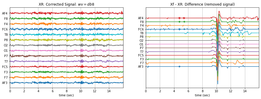
wavelet function¶

#db8
XR = sp.eeg.ATAR_mCh_noParallel(Xf.copy(),wv='db8',beta=0.01,OptMode='elim',verbose=0,)

plt.figure(figsize=(15,5))
plt.subplot(121)
plt.plot(t,XR+np.arange(-7,7)*200)
plt.xlim([t[0],t[-1]])
plt.xlabel('time (sec)')
plt.yticks(np.arange(-7,7)*200,ch_names)
plt.grid()
plt.title('XR: Corrected Signal: '+r'$wv=db8$')

plt.subplot(122)
plt.plot(t,(Xf-XR)+np.arange(-7,7)*200)
plt.xlim([t[0],t[-1]])
plt.xlabel('time (sec)')
plt.yticks(np.arange(-7,7)*200,ch_names)
plt.grid()
plt.title('Xf - XR: Difference (removed signal)')
plt.show()

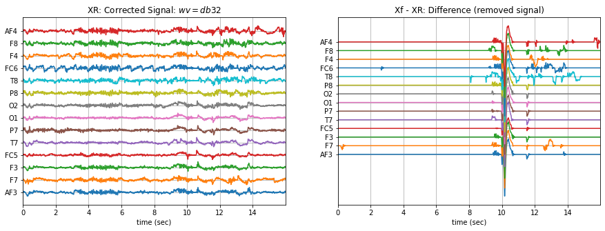
#db32
XR = sp.eeg.ATAR_mCh_noParallel(Xf.copy(),wv='db32',beta=0.01,OptMode='elim',verbose=0,)

plt.figure(figsize=(15,5))
plt.subplot(121)
plt.plot(t,XR+np.arange(-7,7)*200)
plt.xlim([t[0],t[-1]])
plt.xlabel('time (sec)')
plt.yticks(np.arange(-7,7)*200,ch_names)
plt.grid()
plt.title('XR: Corrected Signal: '+r'$wv=db32$')

plt.subplot(122)
plt.plot(t,(Xf-XR)+np.arange(-7,7)*200)
plt.xlim([t[0],t[-1]])
plt.xlabel('time (sec)')
plt.yticks(np.arange(-7,7)*200,ch_names)
plt.grid()
plt.title('Xf - XR: Difference (removed signal)')
plt.show()

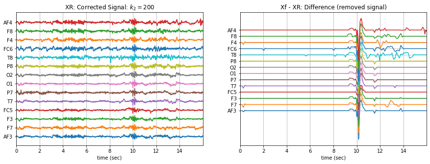
https://raw.githubusercontent.com/Nikeshbajaj/spkit/master/figures/atar_wv_db8.png

https://raw.githubusercontent.com/Nikeshbajaj/spkit/master/figures/atar_wv_db32.png

upper and lower bounds: $k_1$ and $k_2$¶

k1 and k2 are lower and upper bound on the threshold θα. k1 is set to 10, which means, the lowest threshold value will be 10, this helps to prevent the removal of entire signal (zeroing out) due to present of high magnitute of artifact. k2 is largest threshold value, which in terms set the decaying curve of threshold θα. Increasing k2 will make the removal less aggressive

XR = sp.eeg.ATAR_mCh_noParallel(Xf.copy(),wv='db3',beta=0.1,OptMode='elim',verbose=0,k1=10, k2=200)

plt.figure(figsize=(15,5))
plt.subplot(121)
plt.plot(t,XR+np.arange(-7,7)*200)
plt.xlim([t[0],t[-1]])
plt.xlabel('time (sec)')
plt.yticks(np.arange(-7,7)*200,ch_names)
plt.grid()
plt.title('XR: Corrected Signal: '+r'$k_2=200$')

plt.subplot(122)
plt.plot(t,(Xf-XR)+np.arange(-7,7)*200)
plt.xlim([t[0],t[-1]])
plt.xlabel('time (sec)')
plt.yticks(np.arange(-7,7)*200,ch_names)
plt.grid()
plt.title('Xf - XR: Difference (removed signal)')
plt.show()

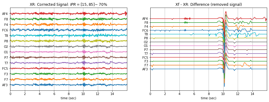
https://raw.githubusercontent.com/Nikeshbajaj/spkit/master/figures/atar_k2_1.png

IPR - Interpercentile range¶

IPR is interpercentile range, which is set to 50% (IPR=[25,75]) as default (inter-quartile range), incresing the range increses the aggressiveness of removing artifacts.

XR = sp.eeg.ATAR_mCh_noParallel(Xf.copy(),wv='db3',beta=0.1,OptMode='elim',verbose=0,k1=10, k2=200, IPR=[15,85])

plt.figure(figsize=(15,5))
plt.subplot(121)
plt.plot(t,XR+np.arange(-7,7)*200)
plt.xlim([t[0],t[-1]])
plt.xlabel('time (sec)')
plt.yticks(np.arange(-7,7)*200,ch_names)
plt.grid()
plt.title('XR: Corrected Signal: '+r'$IPR=[15,85]$~ 70%')

plt.subplot(122)
plt.plot(t,(Xf-XR)+np.arange(-7,7)*200)
plt.xlim([t[0],t[-1]])
plt.xlabel('time (sec)')
plt.yticks(np.arange(-7,7)*200,ch_names)
plt.grid()
plt.title('Xf - XR: Difference (removed signal)')
plt.show()

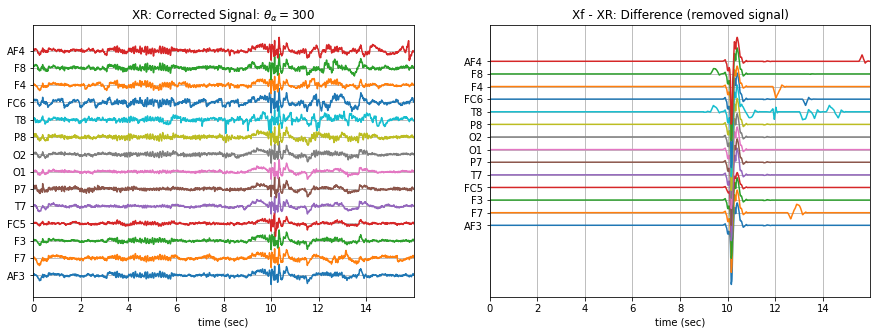
https://raw.githubusercontent.com/Nikeshbajaj/spkit/master/figures/atar_ipr_1.png

constant threshold (θ=300), (not adaptive)¶

fixing threshold (θα=300), not using ipr method to adaptively change threshold¶

Fixing θα with thr_method=None will be applying a fixed threshold in non-adaptive manner, this is effective in the cases where you want to remove the specfic artifacts and leave all the other part of signal untouched. As in following example, only very high peaks are removed and other part of signal is left un-affected.

XR = sp.eeg.ATAR_mCh_noParallel(Xf.copy(),wv='db3',thr_method=None,theta_a=300,OptMode='elim',verbose=0)

plt.figure(figsize=(15,5))
plt.subplot(121)
plt.plot(t,XR+np.arange(-7,7)*200)
plt.xlim([t[0],t[-1]])
plt.xlabel('time (sec)')
plt.yticks(np.arange(-7,7)*200,ch_names)
plt.grid()
plt.title('XR: Corrected Signal: '+r'$\theta_\alpha=300$')

plt.subplot(122)
plt.plot(t,(Xf-XR)+np.arange(-7,7)*200)
plt.xlim([t[0],t[-1]])
plt.xlabel('time (sec)')
plt.yticks(np.arange(-7,7)*200,ch_names)
plt.grid()
plt.title('Xf - XR: Difference (removed signal)')
plt.show()

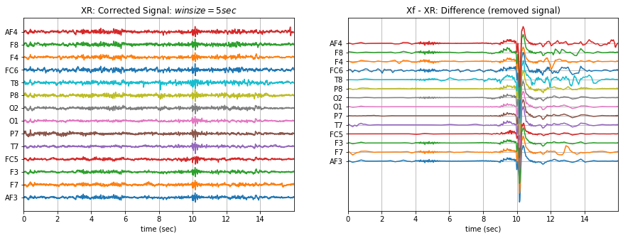
https://raw.githubusercontent.com/Nikeshbajaj/spkit/master/figures/atar_alpha_1.png

window length (5 sec)¶

winsize is be default set to 128 (1 sec), assuming 128 sampling rate, which can be changed as needed. In following example it is changed to 5 sec

XR = sp.eeg.ATAR_mCh_noParallel(Xf.copy(),winsize=128*5,beta=0.01,OptMode='elim',verbose=0,)

plt.figure(figsize=(15,5))
plt.subplot(121)
plt.plot(t,XR+np.arange(-7,7)*200)
plt.xlim([t[0],t[-1]])
plt.xlabel('time (sec)')
plt.yticks(np.arange(-7,7)*200,ch_names)
plt.grid()
plt.title('XR: Corrected Signal: '+r'$winsize=5sec$')

plt.subplot(122)
plt.plot(t,(Xf-XR)+np.arange(-7,7)*200)
plt.xlim([t[0],t[-1]])
plt.xlabel('time (sec)')
plt.yticks(np.arange(-7,7)*200,ch_names)
plt.grid()
plt.title('Xf - XR: Difference (removed signal)')
plt.show()

https://raw.githubusercontent.com/Nikeshbajaj/spkit/master/figures/atar_win_1.png

ATAR - Automatic and Tunable Artifact Removal Algorithm for EEG¶

Notebook¶

View in Jupyter-Notebook ¶

(1) Soft Thresholding (𝛽=0.1) - a quick example¶

(2) Linear Attenuation¶

(3) Elimination¶

Tuning 𝛽 with ‘soft’ : Controlling the aggressiveness¶

Tuning 𝛽 with ‘elim’¶

Tuning 𝛽 with ‘linAtten’¶

Other Settings¶

wavelet function¶

upper and lower bounds: \(k_1\) and \(k_2\)¶

IPR - Interpercentile range¶

constant threshold (θ=300), (not adaptive)¶

fixing threshold (θα=300), not using ipr method to adaptively change threshold¶

window length (5 sec)¶

Table of Contents

Previous topic

Next topic

Quick links

ATAR - Automatic and Tunable Artifact Removal Algorithm for EEG¶

Notebook¶

View in Jupyter-Notebook¶

(1) Soft Thresholding (𝛽=0.1) - a quick example¶

(2) Linear Attenuation¶

(3) Elimination¶

Tuning 𝛽 with ‘soft’ : Controlling the aggressiveness¶

Tuning 𝛽 with ‘elim’¶

Tuning 𝛽 with ‘linAtten’¶

Other Settings¶

wavelet function¶

upper and lower bounds: \(k_1\) and \(k_2\)¶

IPR - Interpercentile range¶

constant threshold (θ=300), (not adaptive)¶

fixing threshold (θα=300), not using ipr method to adaptively change threshold¶

window length (5 sec)¶

View in Jupyter-Notebook ¶