Information Theory for Real-Valued signals

Updating the documentation …

Entropy of signal with finit set of values is easy to compute, since frequency for each value can be computed, however, for real-valued signal it is a little different, because of infinite set of amplitude values. For which spkit comes handy.

*Following Entropy functions compute entropy based the on the sample distribuation, which by default consider process to be IID (Independent Identical Disstribuation) - which means no temporal dependency.*

*For temporal dependency (non-IID) signals, Spectral, Sample, Aproximate, SVD and Dispersion Entropy functions can be used. Which are discribed below*

Entropy of real-valued signal (~ IID)

View in Jupyter-Notebook

import numpy as np
import matplotlib.pyplot as plt
import spkit as sp

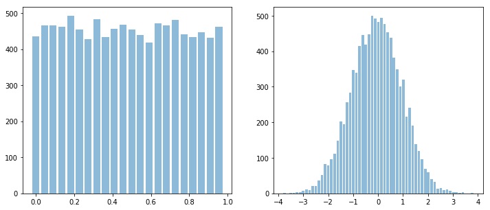
x = np.random.rand(10000)
y = np.random.randn(10000)

plt.figure(figsize=(12,5))
plt.subplot(121)
sp.HistPlot(x,show=False)

plt.subplot(122)
sp.HistPlot(y,show=False)
plt.show()

Shannan entropy

#Shannan entropy
H_x = sp.entropy(x,alpha=1)
H_y = sp.entropy(y,alpha=1)
print('Shannan entropy')
print('Entropy of x: H(x) = ',H_x)
print('Entropy of y: H(y) = ',H_y)

Shannan entropy
Entropy of x: H(x) =  4.4581180171280685
Entropy of y: H(y) =  5.04102391756942

Rényi entropy (e.g. Collision Entropy)

#Rényi entropy
Hr_x= sp.entropy(x,alpha=2)
Hr_y= sp.entropy(y,alpha=2)
print('Rényi entropy')
print('Entropy of x: H(x) = ',Hr_x)
print('Entropy of y: H(y) = ',Hr_y)

Rényi entropy
Entropy of x: H(x) =  4.456806796146617
Entropy of y: H(y) =  4.828391418226062

Mutual Information & Joint Entropy

I_xy = sp.mutual_Info(x,y)
print('Mutual Information I(x,y) = ',I_xy)

H_xy= sp.entropy_joint(x,y)
print('Joint Entropy H(x,y) = ',H_xy)

Joint Entropy H(x,y) =  9.439792556949234
Mutual Information I(x,y) =  0.05934937774825322

Conditional entropy

H_x1y= sp.entropy_cond(x,y)
H_y1x= sp.entropy_cond(y,x)
print('Conditional Entropy of : H(x|y) = ',H_x1y)
print('Conditional Entropy of : H(y|x) = ',H_y1x)

Conditional Entropy of : H(x|y) =  4.398768639379814
Conditional Entropy of : H(y|x) =  4.9816745398211655

Cross entropy & Kullback–Leibler divergence

H_xy_cross= sp.entropy_cross(x,y)
D_xy= sp.entropy_kld(x,y)
print('Cross Entropy of : H(x,y) = :',H_xy_cross)
print('Kullback–Leibler divergence : Dkl(x,y) = :',D_xy)

Cross Entropy of : H(x,y) = : 11.591688735915701
Kullback–Leibler divergence : Dkl(x,y) = : 4.203058010473213

Entropy of real-valued signal (~ non-IID)

Spectral Entropy

Though spectral entropy compute the entropy of frequency components cosidering that frequency distribuation is ~ IID, However, each frquency component has a temporal characterstics, so this is an indirect way to considering the temporal dependency of a signal

H_se = sp.entropy_spectral(x,fs,method='fft')
H_se = sp.entropy_spectral(x,fs,method='welch')

Approximate Entropy

Aproximate Entropy is Embeding based entropy function. Rather than considering a signal sample, it consider the m-continues samples (a m-deminesional temporal pattern) as a symbol generated from a process. This set of “m-continues samples” is considered as “Embeding” and then estimating distribuation of computed symbols (embeddings). In case of a real valued signal, two embeddings will rarely be an exact match, so, the factor r is defined as if two embeddings are less than r distance away to each other, they are considered as same. This is a way to quantization of embedding and limiting the Embedding Space.

For Aproximate Entropy the value of r depends the application and the order (range) of signal. One has to keep in mind that r is the distance be between two Embeddings (m-deminesional temporal pattern). A typical value of r can be estimated on based of SD of x ~ 0.2*std(x).

H_apx = sp.entropy_approx(x,m,r)

Sample Entropy

Sample Entropy is a modified version of Approximate Entropy. m and r are same as in for Approximate entropy

H_sam = sp.entropy_sample(x,m,r)

Singular Value Decomposition Entropy

H_svd = sp.entropy_svd(x,order=3, delay=1)

Permutation Entropy

H_prm = sp.entropy_permutation(x,order=3, delay=1)

Dispersion Entropy

check here (https://spkit.readthedocs.io/en/latest/dispersion_entropy.html)

---

EEG Signal

View in Jupyter-Notebook

Single Channel

import numpy as np
import matplotlib.pyplot as plt
import spkit as sp
from spkit.data import load_data
print(sp.__version__)

# load sample of EEG segment
X,ch_names = load_data.eegSample()
t = np.arange(X.shape[0])/128
nC = len(ch_names)


x1 =X[:,0] #'AF3' - Frontal Lobe
x2 =X[:,6] #'O1'  - Occipital Lobe
#Shannan entropy
H_x1= sp.entropy(x1,alpha=1)
H_x2= sp.entropy(x2,alpha=1)

#Rényi entropy
Hr_x1= sp.entropy(x1,alpha=2)
Hr_x2= sp.entropy(x2,alpha=2)

print('Shannan entropy')
print('Entropy of x1: H(x1) =\t ',H_x1)
print('Entropy of x2: H(x2) =\t ',H_x2)
print('-')
print('Rényi entropy')
print('Entropy of x1: H(x1) =\t ',Hr_x1)
print('Entropy of x2: H(x2) =\t ',Hr_x2)
print('-')

Multi-Channels (cross)

#Joint entropy
H_x12= sp.entropy_joint(x1,x2)

#Conditional Entropy
H_x12= sp.entropy_cond(x1,x2)
H_x21= sp.entropy_cond(x2,x1)

#Mutual Information
I_x12 = sp.mutual_Info(x1,x2)

#Cross Entropy
H_x12_cross= sp.entropy_cross(x1,x2)

#Diff Entropy
D_x12= sp.entropy_kld(x1,x2)

print('Joint Entropy H(x1,x2) =\t',H_x12)
print('Mutual Information I(x1,x2) =\t',I_x12)
print('Conditional Entropy of : H(x1|x2) =\t',H_x12)
print('Conditional Entropy of : H(x2|x1) =\t',H_x21)
print('-')
print('Cross Entropy of : H(x1,x2) =\t',H_x12_cross)
print('Kullback–Leibler divergence : Dkl(x1,x2) =\t',D_x12)


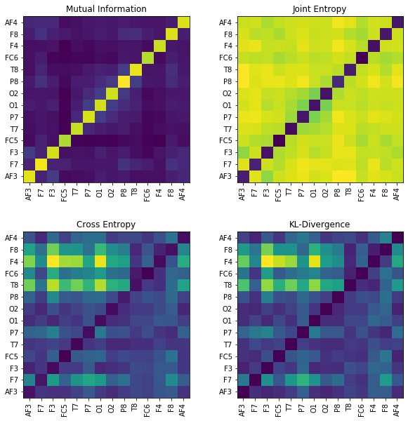
MI = np.zeros([nC,nC])
JE = np.zeros([nC,nC])
CE = np.zeros([nC,nC])
KL = np.zeros([nC,nC])
for i in range(nC):
    x1 = X[:,i]
    for j in range(nC):
        x2 = X[:,j]

        #Mutual Information
        MI[i,j] = sp.mutual_Info(x1,x2)

        #Joint entropy
        JE[i,j]= sp.entropy_joint(x1,x2)

        #Cross Entropy
        CE[i,j]= sp.entropy_cross(x1,x2)

        #Diff Entropy
        KL[i,j]= sp.entropy_kld(x1,x2)



  plt.figure(figsize=(10,10))
  plt.subplot(221)
  plt.imshow(MI,origin='lower')
  plt.yticks(np.arange(nC),ch_names)
  plt.xticks(np.arange(nC),ch_names,rotation=90)
  plt.title('Mutual Information')
  plt.subplot(222)
  plt.imshow(JE,origin='lower')
  plt.yticks(np.arange(nC),ch_names)
  plt.xticks(np.arange(nC),ch_names,rotation=90)
  plt.title('Joint Entropy')
  plt.subplot(223)
  plt.imshow(CE,origin='lower')
  plt.yticks(np.arange(nC),ch_names)
  plt.xticks(np.arange(nC),ch_names,rotation=90)
  plt.title('Cross Entropy')
  plt.subplot(224)
  plt.imshow(KL,origin='lower')
  plt.yticks(np.arange(nC),ch_names)
  plt.xticks(np.arange(nC),ch_names,rotation=90)
  plt.title('KL-Divergence')
  plt.subplots_adjust(hspace=0.3)
  plt.show()

---